TidyTuesday Measles Vaccination Data
There is a Github repo td20200225.
I had to spend more time than expected on data cleaning.
The analysis is done in R with a tidy work flow.
This is my first #tidytuesday project. My work flow isn’t settled.
Note - I don’t know the US American system. So I speculate on some correlations. Mostly I suppose they don’t do vaccination against the parents will, but rather I’m seeing honest typos in the data. Not too motivated to organized secondary sources.
Setup
library(ggplot2)
library(dplyr)
##
## Attaching package: 'dplyr'
## The following objects are masked from 'package:stats':
##
##     filter, lag
## The following objects are masked from 'package:base':
##
##     intersect, setdiff, setequal, union
library(tidyr)
library(pander)
knitr::opts_chunk$set(warning = FALSE, message=FALSE)
# library(svglite)
# knitr::opts_chunk$set(
#   dev = "svglite",
#   fig.ext = ".svg"
# )
measles <- readRDS("data/measles.RDS")
cmeasles  <- measles %>% filter(!suspicious)
checking data
I notice some annoyances:
- In some columns
-1is used instead ofNA - Religious refusal is boolean ?!?
- Lots of missing values.
- The ratios of vaccinations and students refusing don’t add up.
- In one school
160%(Montessori At Samish Woods) refused for personal reasons - also has yearnull.
Data structure
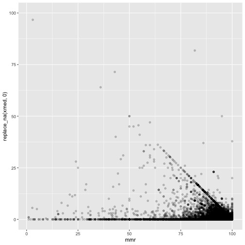
ptm <- proc.time()
ggplot(measles, mapping=aes(x=mmr, y=replace_na(xmed,0))) +
  geom_point(alpha = 0.2)
proc.time()-ptm
##    user  system elapsed
##   0.811   0.050   1.144
ggplot(measles, mapping=aes(x=mmr, y=replace_na(xper,0))) +
  geom_point(alpha = 0.2)
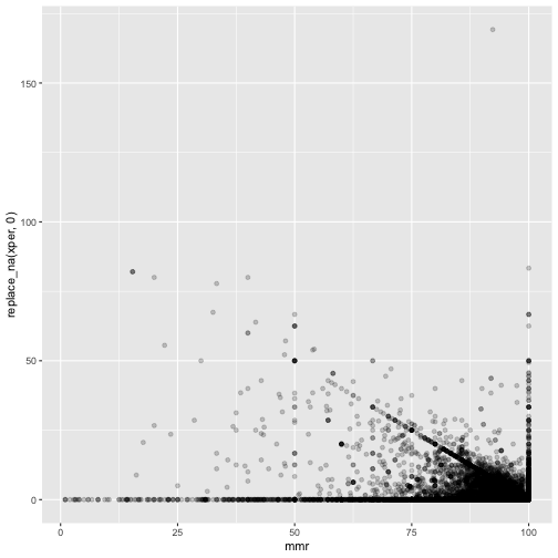
These are suspicious. There is a clearly a diagonal line visible.
There should not be points above - either they withdrew the consent, or were wrongly reported vaccinated.
It seems many just report 100%.
And the magic school where 169% rejected - on the figure this looks like a reasonable typo - 16.9% may fit. But still the mmr is 92.3% - way too high.
susps <- measles %>% filter(suspicious) %>% select(-lng,-lat)
In total there are 1844 suspicious entries - that’s not much compared out of 66113.
Imputation
I didn’t want to exclude all the NAs.
xmed and xper
These seem simple. They are NA for 100% schools.
So in most cases the NA just may be 0.
xrel
This is harder as it is not numerically reported. But mmr and xmed seem to be reliable - so I decided to have all unexplained non-vaccinating together. Of course this will group religious with all where no explanation was required.
School type
School type seemets interesting, but has lots of NAs.
Seems the reason is most states don’t report these.
Not much I can do there.
pandoc.table(measles %>% group_by(type, state) %>% summarise(n=n()) %>%
       spread(type,n),
     caption = "types of school vs. states",
     style="rmarkdown",
     split.tables = Inf)
| state | BOCES | Charter | Kindergarten | Nonpublic | Private | Public | |
|---|---|---|---|---|---|---|---|
| Arizona | NA | 276 | NA | NA | 224 | 951 | NA |
| Arkansas | NA | NA | NA | NA | NA | NA | 567 |
| California | NA | NA | NA | NA | 2745 | 13353 | NA |
| Colorado | NA | NA | 1488 | NA | 21 | NA | NA |
| Connecticut | NA | NA | NA | 173 | NA | 622 | NA |
| Florida | NA | NA | NA | NA | NA | NA | 2678 |
| Idaho | NA | NA | NA | NA | NA | NA | 475 |
| Illinois | NA | NA | NA | NA | NA | NA | 7686 |
| Iowa | NA | NA | NA | NA | NA | NA | 1370 |
| Maine | NA | NA | NA | NA | NA | NA | 357 |
| Massachusetts | NA | NA | NA | NA | 486 | 1108 | NA |
| Michigan | NA | NA | NA | NA | NA | NA | 2351 |
| Minnesota | NA | NA | NA | NA | NA | NA | 1813 |
| Missouri | NA | NA | NA | NA | NA | NA | 748 |
| Montana | NA | NA | NA | NA | NA | NA | 645 |
| New Jersey | NA | NA | NA | NA | NA | NA | 2211 |
| New York | 47 | NA | NA | NA | 2294 | 1934 | NA |
| North Carolina | NA | NA | NA | NA | NA | NA | 2085 |
| North Dakota | NA | NA | NA | NA | NA | NA | 387 |
| Ohio | NA | NA | NA | NA | 1012 | 2153 | NA |
| Oklahoma | NA | NA | NA | NA | NA | NA | 1249 |
| Oregon | NA | NA | NA | NA | NA | NA | 817 |
| Pennsylvania | NA | NA | NA | NA | NA | NA | 1939 |
| Rhode Island | NA | NA | NA | NA | NA | NA | 230 |
| South Dakota | NA | NA | NA | NA | NA | NA | 390 |
| Tennessee | NA | NA | NA | NA | NA | NA | 1152 |
| Texas | NA | NA | NA | NA | NA | NA | 811 |
| Utah | NA | NA | NA | NA | 33 | 571 | NA |
| Vermont | NA | NA | NA | NA | NA | NA | 349 |
| Virginia | NA | NA | NA | NA | NA | NA | 1468 |
| Washington | NA | NA | NA | NA | NA | NA | 2221 |
| Wisconsin | NA | NA | NA | NA | NA | NA | 2623 |
Table: types of school vs. states
Enroll
Number of students would be useful for a weighted average.
pander(measles %>% group_by( state) %>%
       summarise(median=median(enroll, na.rm = T),
		 mad = mad(enroll, na.rm = T)),
       caption = "types of school vs. states",
       split.tables = Inf,
       style="rmarkdown")
| state | median | mad |
|---|---|---|
| Arizona | 71 | 29.65 |
| Arkansas | 505 | 192.7 |
| California | 77 | 43 |
| Colorado | 52 | 34.1 |
| Connecticut | NA | NA |
| Florida | 89 | 35.58 |
| Idaho | NA | NA |
| Illinois | 333 | 206.1 |
| Iowa | 270 | 179.4 |
| Maine | 30 | 28.17 |
| Massachusetts | NA | NA |
| Michigan | 58 | 35.58 |
| Minnesota | 56 | 48.93 |
| Missouri | NA | NA |
| Montana | 196 | 180.9 |
| New Jersey | 45 | 40.03 |
| New York | NA | NA |
| North Carolina | 63 | 44.48 |
| North Dakota | 32.5 | 28.91 |
| Ohio | 51 | 34.1 |
| Oklahoma | NA | NA |
| Oregon | 58 | 29.65 |
| Pennsylvania | 63 | 31.13 |
| Rhode Island | 46 | 31.13 |
| South Dakota | 19 | 23.72 |
| Tennessee | 71 | 37.06 |
| Texas | NA | NA |
| Utah | 498 | 201.6 |
| Vermont | 107 | 106.7 |
| Virginia | 72 | 41.51 |
| Washington | NA | NA |
| Wisconsin | NA | NA |
Table: types of school vs. states
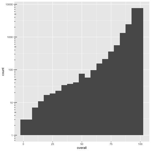
The overall median is 80 and mad 56.3388. I chose 100 as guess for the undocumented ones so that there would be a nice log10.
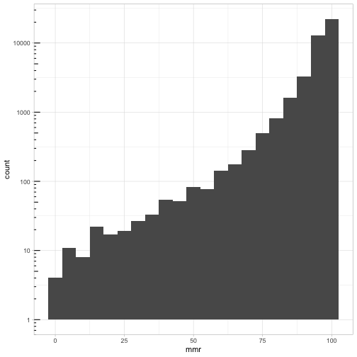
ggplot(cmeasles, mapping=aes(x=mmr)) +
  geom_histogram(binwidth=5) +
  scale_y_log10() + annotation_logticks(sides=c("l")) +
  theme_light()
ggplot(cmeasles, mapping=aes(x=overall)) +
  geom_histogram(binwidth=5) +
  scale_y_log10() + annotation_logticks(sides=c("l"))
ggplot(measles, mapping=aes(x=overall, y=mmr)) +
  geom_point(alpha = 0.2)
xrel is boolean!
ggplot(cmeasles, mapping=aes(x=mmr)) +
  geom_histogram(binwidth=5) +
  scale_y_log10() + annotation_logticks(sides=c("l"))
It should be mmr + xmed < 100!
ggplot(cmeasles, mapping=aes(y=mmr, x=xmed)) +
  geom_point()
cmeasles %>% filter(xmed > 50)
## # A tibble: 2 x 18
##   index state year  name  type  city  county district enroll   mmr overall xrel
##   <dbl> <chr> <chr> <chr> <chr> <chr> <chr>  <lgl>     <dbl> <dbl>   <dbl> <lgl>
## 1  6500 Cali… 2018… Yuba… Publ… Neva… Nevada NA           64    36      36 NA
## 2   827 Mass… 2018… Rudo… Priv… Grea… Berks… NA           NA     3      NA NA
## # … with 6 more variables: xmed <dbl>, xper <dbl>, lat <dbl>, lng <dbl>,
## #   maxknownexcl <dbl>, suspicious <lgl>
ggplot(cmeasles, mapping=aes(y=mmr, x=xper)) +
  geom_point()

cmeasles %>% filter(xmed > 50)
## # A tibble: 2 x 18
##   index state year  name  type  city  county district enroll   mmr overall xrel
##   <dbl> <chr> <chr> <chr> <chr> <chr> <chr>  <lgl>     <dbl> <dbl>   <dbl> <lgl>
## 1  6500 Cali… 2018… Yuba… Publ… Neva… Nevada NA           64    36      36 NA
## 2   827 Mass… 2018… Rudo… Priv… Grea… Berks… NA           NA     3      NA NA
## # … with 6 more variables: xmed <dbl>, xper <dbl>, lat <dbl>, lng <dbl>,
## #   maxknownexcl <dbl>, suspicious <lgl>
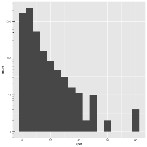
ggplot(cmeasles, mapping=aes(x=xper)) +
  geom_histogram(binwidth=5) +
  scale_y_log10() + annotation_logticks(sides=c("l"))
ggplot(cmeasles, mapping=aes(x=xper,y=mmr)) +
  geom_point()
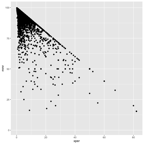
Note:
- has only one sample per school.
- only 15 states
cmeasles %>% group_by(type) %>% summarise(n=n())%>% arrange(-n)
## # A tibble: 7 x 2
##   type             n
##   <chr>        <int>
## 1 Public       19090
## 2 <NA>         17625
## 3 Private       4424
## 4 Kindergarten   959
## 5 Charter        155
## 6 BOCES           43
## 7 Nonpublic       17
Lots of unlabelled. Private don’t play much of a role.
cmeasles %>% group_by(state) %>% summarise(n=n(),enrolls = sum(enroll, na.rm=T)) %>% arrange(-n)
## # A tibble: 21 x 3
##    state            n enrolls
##    <chr>        <int>   <dbl>
##  1 California   14033 1216297
##  2 Illinois      7619 2653668
##  3 New York      3942       0
##  4 Ohio          2915  176867
##  5 Pennsylvania  1939  138722
##  6 Washington    1793       0
##  7 Minnesota     1590   93114
##  8 Colorado       966   51641
##  9 Arizona        887   61983
## 10 Texas          811       0
## # … with 11 more rows
Everything is dwarfed by California and Illinois.
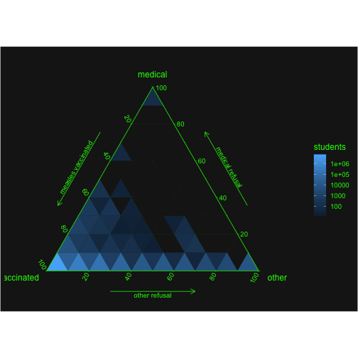
Visualisierung:
Idea ternary plot:
library(ggtern)
cm2 <- cmeasles %>%
  mutate(xmed = replace_na(xmed,0),
	 xother = 100 - mmr - xmed,
	 enroll = replace_na(enroll,100)) %>%
  mutate_at(vars(mmr, xmed, xother), ~./100)
cms <- sample_n(cm2,100)

my_breaks  <-  10^seq(2,6)
ptm <- proc.time()
ggtern(cm2, aes(mmr,xmed,xother)) +
  geom_tri_tern(bins = 10, aes(fill=..stat.., value=enroll), fun=function(z){(sum(z))}) +
  scale_L_continuous("vaccinated") +
  Llab("measles vaccinated") +
  scale_R_continuous("other") +
  Rlab("other refusal") +
  scale_T_continuous("medical") +
  Tlab("medical refusal") +
  scale_fill_gradient(name = "students", trans = "log10",
		      breaks = my_breaks, labels = my_breaks,
		      na.value = "gray10") +
  theme_matrix() +
  theme(legend.background = element_rect(fill = "gray10"))
  # theme_tropical()
  #theme_linedraw()
  #theme_bvbg()
  # scale_fill_continuous(low="thistle2", high="darkred",
  #                      guide="colorbar",na.value="white") +
proc.time()-ptm
##    user  system elapsed
##   1.254   0.131   1.399